Una solución para la multicolinealidad en modelos de función de producción de frontera estocástica
DOI:
https://doi.org/10.17533/udea.le.n86a01Palabras clave:
análisis de frontera estocástica, eficiencia técnica, productividad, multicolinealidad, estimación de componentes principales.Resumen
Este artículo considera el problema de colinealidad entre insumos en un modelo de producción de frontera estocástica, un tema que ha recibido poca atención en la literatura econométrica. Para abordar el problema, se propone una solución basada en componentes principales que permite interpretar conjuntamente la eficiencia técnica y los parámetros de tecnología del modelo. Los resultados de la aplicación del método con datos simulados y reales muestran que éste es fácil de usar y presenta un buen desempeño.
Descargas
Citas
Aigner, Dennis; Lovell, Knox & Schmidt, Peater (1977). “Formulation and estimation of stochastic frontier production function models”, Journal of Econometrics, Vol. 6, Issue 1, pp. 21-37.
Belsley, David; Kuh, Edwin & Welsh, Roy (1980). Regression Diagnostics: Identifying Influential Data and Sources of Collinearity. New York: John Wiley & Sons, Inc.
Coelli, Timothy & Henningsen, Arne (2013). Frontier: Stochastic Frontier Analysis. Retrieved from: http://CRAN.R-Project.org/package=frontier. R package version 1.1-0. (Accessed on July 2014).
Coelli, Timothy; Rao, Prasada D.S.; O’Donnell, Christopher J. & Battese, George E. (2005). An Introduction to Efficiency and Productivity Analysis (2nd. Ed.). New York: Springer.
Filippini, Massimo; Hrovatin, Nevenka & Zoric, Jelena (2008). “Cost efficiency of slovenian water distribution utilities: an application of stochastic frontier methods”, Journal of Productivity Analysis, Vol. 29. Issue 2, pp. 169-182.
Fomby, Thomas B.; Johnson, Stanley R. & Hill, Carter (1984). Advanced Econometric Methods. New York: Springer.
Greene, William (1980a). “Maximum likelihood estimation of econometric frontier functions”, Journal of Econometrics, Vol. 13, Issue 1, pp. 27-56.
Greene, William (1980b). “On the estimation of a flexible frontier production model”, Journal of Econometrics, Vol. 13, Issue 1, pp. 101-115.
Greene, William (2008). “The econometric approach to efficiency analysis”. In: Fried, Harold; Lovell, Knox & Schmidt, Shelton (Eds.), The Measurement of Productive Efficiency and Productivity Growth (pp. 92-150). New York, Oxford University Press.
Groß, Jürgen (2003). “Linear Regression”, Lecture Notes in Statistics, Vol. 75. Springer.
Hwang, Gene J. T. & Nettleton, Dan (2003). “Principal components regression with data chosen components and related methods”, Technometrics, Vol. 45, No. 1, pp. 70-79.
Jolliffe, Ian T. (1982). “A note on the use of principal components in regression”, Journal of the Royal Statistical Society. Series C (Applied Statistics), Vol. 31, No. 3, pp. 300-303.
Jolliffe, Ian T. (2002). Principal Component Analysis (2nd Ed.). New York: Springer.
Kumbhakar, Subal C. & Lovell, C. Knox (2000). Stochastic Frontier Analysis. Cambridge: Cambridge University Press.
Mason, Robert & Gunst, Richard (1985). “Selecting principal components in regression”, Statistics and Probability Letters, Vol. 3, Issue 6, pp. 299-301.
Massy, William F. (1965). “Principal components regression in exploratory
statistical research”, Journal of the American Statistical Association, Vol. 60, Issue 309, pp. 234-256.
Meeusen, Wim & van Den Broeck, Julien (1977). “Efficiency estimation from Cobb-Douglas production functions with composed error”, International Economic Review, Vol. 18, No. 2, pp. 435-444.
Puig-Junoy, Jaume (2001). “Technical inefficiency and public capital in U.S. states: A stochastic frontier approach”, Journal of Regional Science, Vol. 41, Issue 1, pp. 75-96.
Stevenson, Rodney (1980). “Likelihood functions for generalized stochastic frontier estimation”, Journal of Econometrics, Vol. 13, Issue 1, pp. 58-66.
Descargas
Publicado
Cómo citar
Número
Sección
Licencia
Derechos de autor 2017 Elkin Castaño, Santiago Gallón

Esta obra está bajo una licencia internacional Creative Commons Atribución-NoComercial-CompartirIgual 4.0.
Este sitio web, por Universidad de Antioquia, está licenciado bajo una Creative Commons Attribution License.
Los autores que publiquen en esta revista aceptan que conservan los derechos de autor y ceden a la revista el derecho de la primera publicación, con el trabajo registrado con una Licencia de Atribución-NoComercial-CompartirIgual de Creative Commons, que permite a terceros utilizar lo publicado siempre que mencionen su autoría y a la publicación original en esta revista.
Los autores pueden realizar acuerdos contractuales independientes y adicionales para la distribución no exclusiva de la versión del trabajo publicada en la revista (por ejemplo, incluirla en un repositorio institucional o publicarla en un libro) siempre que sea con fines no comerciales y se reconozca de manera clara y explícita que el artículo ha sido originalmente publicado en esta revista.
Se permite y recomienda a los autores publicar sus artículos en Internet (por ejemplo, en páginas institucionales o personales), ya que puede conducir a intercambios provechosos y a una mayor difusión y citación de los trabajos publicados.


 (
( represent the deterministic and noise components of the frontier respectively, xi
⊤
β + vi
is the maximum output reached by the firm which constitutes the stochastic frontier, and ui
is the non-negative random technical inefficiency component (i.e., the amount by which the firm fails to achieve its optimum). A symmetric distribution, such as the normal distribution, is usually assumed for vi. It is also common to assume that vi
and ui
are independent, and that both errors are uncorre lated with xi
. Typically, the production function relies on a Cobb-Douglas, translog, or any other logarithmic production model log(yi)= xi
⊤
β + vi
- ui
, where the components of xi
are logarithms of inputs, its squares and cross products.
  (
( (
( Therefore, the strategy consists in preventing that the estimate goes in directions λipj
associated to fairly small λj
(see
 Thus, the principal component estimator of β in (2) is given by
  (
(
 (
( where σ
u = 3, σ
v = 2.5, σ
2 = σ
2
u + σ
2
v = 15.25, r = σ
2
u/σ
2 =0.59, (β
0, β
1, β
2) = (1, 0.8, 0.7); and (x
1, x
2) ~ N (µ, Σ) with µ = (20, 25) and
Σ
=
DRD
, where
D
= diag(σ
x1 , σ
x2 )= diag(1, 2); and
  with ρ = Corr(x1,x2) = 0.7, 0.8, 0.9. For the most severe multicollinearity prob lem, where ρ = 0.9, we performed the simulations with n = 1000 to study the large sample properties of the estimator. We used the frontier: Stochastic Frontier Analysis R package version 1.1-0 by
  and the usual stochastic frontier analysis
  methods for the assumed values of ρ. Results indicate that, in general, the coefficient estimators obtained with the principal-component-based method are biased, as these biases do not decrease asymptotically. However, the estimators have less MSE with respect to the ones obtained by the traditional method, even in large samples. The usual estimators are biased for finite samples with greater biases than for the proposed method, although these decrease asymptotically. The estimations for γ and σ
2 remain unaffected if the principal components are chosen correctly. Finally, when keeping fixed the number of principal components, the biases increase as the linear relationship among variables decreases.
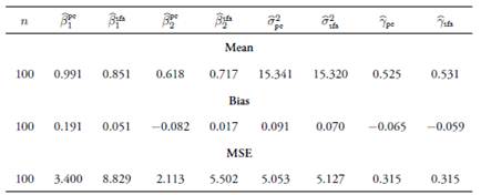
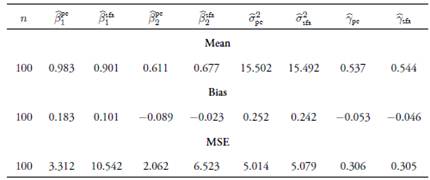
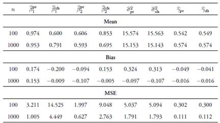
 Estimations were carried out us ing the LIMited DEPendent −LIMDEP− econometric software (version 10). As can be seen in
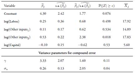

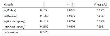
 remains are correct, the proposed method. Furthermore, when keeping fixed the number of prin cipal components, the biases of the proposed estimator increase as the linear relation between covariates decreases. The choice of the number of principal components is critical to the estimation of β, γ and σ2, as well as for the efficiency component. After applying the proposed method on real data from the agricultural and livestock sectors to evaluate its tech