
A solution for multicollinearity in stochastic frontier production function models
DOI:
https://doi.org/10.17533/udea.le.n86a01Keywords:
stochastic frontier analysis, technical efficiency, productivity, multicollinearity, principal component estimation.Abstract
This paper considers the problem of collinearity among inputs in a stochastic frontier production model, an issue that has received little attention in the econometric literature. To address this problem, a principal-component-based solution is proposed, which allows carrying out a joint interpretation of technical efficiency and the technology parameters of the model. Applications of the method to simulated and real data show its usability and effective performance.
Downloads
References
Aigner, Dennis; Lovell, Knox & Schmidt, Peater (1977). “Formulation and estimation of stochastic frontier production function models”, Journal of Econometrics, Vol. 6, Issue 1, pp. 21-37.
Belsley, David; Kuh, Edwin & Welsh, Roy (1980). Regression Diagnostics: Identifying Influential Data and Sources of Collinearity. New York: John Wiley & Sons, Inc.
Coelli, Timothy & Henningsen, Arne (2013). Frontier: Stochastic Frontier Analysis. Retrieved from: http://CRAN.R-Project.org/package=frontier. R package version 1.1-0. (Accessed on July 2014).
Coelli, Timothy; Rao, Prasada D.S.; O’Donnell, Christopher J. & Battese, George E. (2005). An Introduction to Efficiency and Productivity Analysis (2nd. Ed.). New York: Springer.
Filippini, Massimo; Hrovatin, Nevenka & Zoric, Jelena (2008). “Cost efficiency of slovenian water distribution utilities: an application of stochastic frontier methods”, Journal of Productivity Analysis, Vol. 29. Issue 2, pp. 169-182.
Fomby, Thomas B.; Johnson, Stanley R. & Hill, Carter (1984). Advanced Econometric Methods. New York: Springer.
Greene, William (1980a). “Maximum likelihood estimation of econometric frontier functions”, Journal of Econometrics, Vol. 13, Issue 1, pp. 27-56.
Greene, William (1980b). “On the estimation of a flexible frontier production model”, Journal of Econometrics, Vol. 13, Issue 1, pp. 101-115.
Greene, William (2008). “The econometric approach to efficiency analysis”. In: Fried, Harold; Lovell, Knox & Schmidt, Shelton (Eds.), The Measurement of Productive Efficiency and Productivity Growth (pp. 92-150). New York, Oxford University Press.
Groß, Jürgen (2003). “Linear Regression”, Lecture Notes in Statistics, Vol. 75. Springer.
Hwang, Gene J. T. & Nettleton, Dan (2003). “Principal components regression with data chosen components and related methods”, Technometrics, Vol. 45, No. 1, pp. 70-79.
Jolliffe, Ian T. (1982). “A note on the use of principal components in regression”, Journal of the Royal Statistical Society. Series C (Applied Statistics), Vol. 31, No. 3, pp. 300-303.
Jolliffe, Ian T. (2002). Principal Component Analysis (2nd Ed.). New York: Springer.
Kumbhakar, Subal C. & Lovell, C. Knox (2000). Stochastic Frontier Analysis. Cambridge: Cambridge University Press.
Mason, Robert & Gunst, Richard (1985). “Selecting principal components in regression”, Statistics and Probability Letters, Vol. 3, Issue 6, pp. 299-301.
Massy, William F. (1965). “Principal components regression in exploratory
statistical research”, Journal of the American Statistical Association, Vol. 60, Issue 309, pp. 234-256.
Meeusen, Wim & van Den Broeck, Julien (1977). “Efficiency estimation from Cobb-Douglas production functions with composed error”, International Economic Review, Vol. 18, No. 2, pp. 435-444.
Puig-Junoy, Jaume (2001). “Technical inefficiency and public capital in U.S. states: A stochastic frontier approach”, Journal of Regional Science, Vol. 41, Issue 1, pp. 75-96.
Stevenson, Rodney (1980). “Likelihood functions for generalized stochastic frontier estimation”, Journal of Econometrics, Vol. 13, Issue 1, pp. 58-66.

Published
How to Cite
Issue
Section
License
Copyright (c) 2017 Elkin Castaño, Santiago Gallón

This work is licensed under a Creative Commons Attribution-NonCommercial-ShareAlike 4.0 International License.
This page, by Universidad de Antioquia, is licensed under a Creative Commons Attribution License.
Authors who publish with this journal agree to retain copyright and grant the journal right of first publication, with the article licensed under a Creative Commons Attribution-NonCommercial-ShareAlike License allowing others to share it as long as they acknowledge its authorship and original publication in this journal.
Authors can enter into separate, additional contractual arrangements for the non-exclusive distribution of the journal's published version of the work (e.g., post it to an institutional repository or publish it in a book), provided that these arrangements be not for profit and the journal be acknowledged as the original source of publication.
Authors are permitted and encouraged to post their papers online (e.g., in institutional repositories or on their websites), as it can lead to valuable exchanges as well as greater citation of the published work.


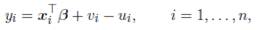 (
( represent the deterministic and noise components of the frontier respectively, xi
⊤
β + vi
is the maximum output reached by the firm which constitutes the stochastic frontier, and ui
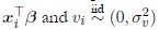
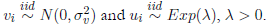
is the non-negative random technical inefficiency component (i.e., the amount by which the firm fails to achieve its optimum). A symmetric distribution, such as the normal distribution, is usually assumed for vi. It is also common to assume that vi
and ui
are independent, and that both errors are uncorre lated with xi
. Typically, the production function relies on a Cobb-Douglas, translog, or any other logarithmic production model log(yi)= xi
⊤
β + vi
- ui
, where the components of xi
are logarithms of inputs, its squares and cross products.
represent the deterministic and noise components of the frontier respectively, xi
⊤
β + vi
is the maximum output reached by the firm which constitutes the stochastic frontier, and ui
is the non-negative random technical inefficiency component (i.e., the amount by which the firm fails to achieve its optimum). A symmetric distribution, such as the normal distribution, is usually assumed for vi. It is also common to assume that vi
and ui
are independent, and that both errors are uncorre lated with xi
. Typically, the production function relies on a Cobb-Douglas, translog, or any other logarithmic production model log(yi)= xi
⊤
β + vi
- ui
, where the components of xi
are logarithms of inputs, its squares and cross products.  (
( (
( Therefore, the strategy consists in preventing that the estimate goes in directions λipj
associated to fairly small λj
(see
Therefore, the strategy consists in preventing that the estimate goes in directions λipj
associated to fairly small λj
(see 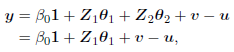
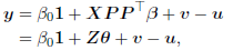
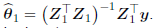 Thus, the principal component estimator of β in (2) is given by
  (
(
 (
(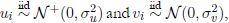 where σ
u = 3, σ
v = 2.5, σ
2 = σ
2
u + σ
2
v = 15.25, r = σ
2
u/σ
2 =0.59, (β
0, β
1, β
2) = (1, 0.8, 0.7); and (x
1, x
2) ~ N (µ, Σ) with µ = (20, 25) and
Σ
=
DRD
, where
D
= diag(σ
x1 , σ
x2 )= diag(1, 2); and
where σ
u = 3, σ
v = 2.5, σ
2 = σ
2
u + σ
2
v = 15.25, r = σ
2
u/σ
2 =0.59, (β
0, β
1, β
2) = (1, 0.8, 0.7); and (x
1, x
2) ~ N (µ, Σ) with µ = (20, 25) and
Σ
=
DRD
, where
D
= diag(σ
x1 , σ
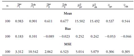
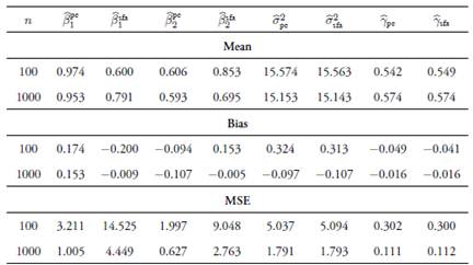
x2 )= diag(1, 2); and  with ρ = Corr(x1,x2) = 0.7, 0.8, 0.9. For the most severe multicollinearity prob lem, where ρ = 0.9, we performed the simulations with n = 1000 to study the large sample properties of the estimator. We used the frontier: Stochastic Frontier Analysis R package version 1.1-0 by
  and the usual stochastic frontier analysis
  methods for the assumed values of ρ. Results indicate that, in general, the coefficient estimators obtained with the principal-component-based method are biased, as these biases do not decrease asymptotically. However, the estimators have less MSE with respect to the ones obtained by the traditional method, even in large samples. The usual estimators are biased for finite samples with greater biases than for the proposed method, although these decrease asymptotically. The estimations for γ and σ
2 remain unaffected if the principal components are chosen correctly. Finally, when keeping fixed the number of principal components, the biases increase as the linear relationship among variables decreases.
methods for the assumed values of ρ. Results indicate that, in general, the coefficient estimators obtained with the principal-component-based method are biased, as these biases do not decrease asymptotically. However, the estimators have less MSE with respect to the ones obtained by the traditional method, even in large samples. The usual estimators are biased for finite samples with greater biases than for the proposed method, although these decrease asymptotically. The estimations for γ and σ
2 remain unaffected if the principal components are chosen correctly. Finally, when keeping fixed the number of principal components, the biases increase as the linear relationship among variables decreases. 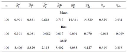
 Estimations were carried out us ing the LIMited DEPendent −LIMDEP− econometric software (version 10). As can be seen in
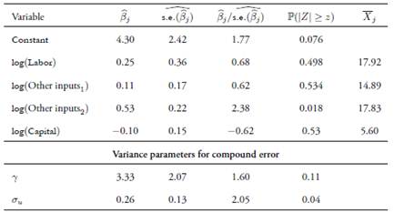
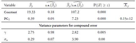
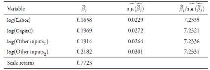
 remains are correct, the proposed method. Furthermore, when keeping fixed the number of prin cipal components, the biases of the proposed estimator increase as the linear relation between covariates decreases. The choice of the number of principal components is critical to the estimation of β, γ and σ2, as well as for the efficiency component. After applying the proposed method on real data from the agricultural and livestock sectors to evaluate its tech